


Photo by Nick Fewings on Unsplash
Determine handwritten digits using Neural Network
Part 2 : End-to-End Implementation using TensorFlow


Introduction
Finally, as the Prince was promised, this blog was also promised tons of weeks back and here it is.
Part 2 : End-to-End Implementation using TensorFlow for determining handwritten digits.
Previously on Part 1: The Concept, we have looked upon the conceptual part of the architecture of neural network, how it's layers are designed and how it learns. This blog will be more on technical side to transform those conceptual part into actual implementation and see our results.
Spoiler : In the process of building our neural network model, we'll be touching some concepts like Normalization, Tuning our model, Learning Rate of Optimizer function and much more... So keep reading. Thanks 🙂
I'll be following the same workflow that we saw in our previous blog on Machine Learning Workflow.
Let me drop the screenshot here for a quick recap.
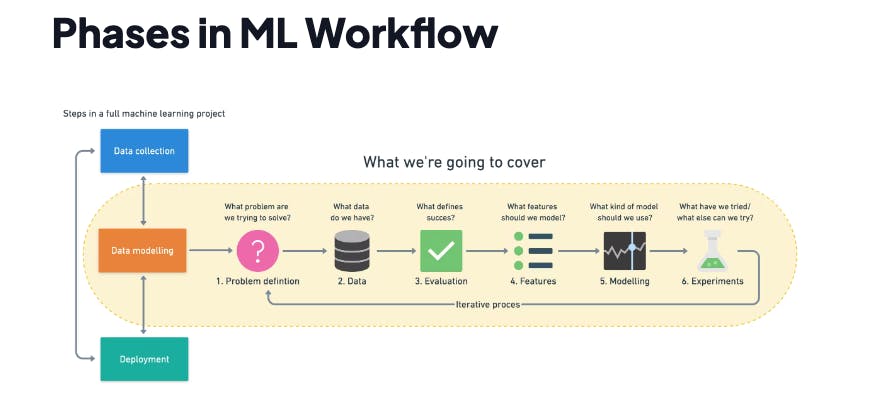
So let's start with Problem Definition.
Problem Definition
Recognise(identify) handwritten digits, from mnist dataset which contains B&W images of each digit written on 28x28 pixel box.
How to do problem definition? Check this out
Data
The data we're using is officially provided by The MNIST DATABASE but thankfully we have TensorFlow dataset which we can use directly by importing it into our notebook.
The digits have been sized-normalized and centered in a fixed-sized image.
The data is quite preprocessed and well-formatted.
Evaluation
Our goal is to achieve Accuracy above 95%.
Features
Some information about the data,
- We're dealing with images(unstructured data) so it's probably best we use deep learning/transfer learning technique to solve this problem.
- There are around a 60,000 examples of training set.
- There are around a 10,000 examples of test set.
The Actual Start
Enough talk, lets get our hands dirty by getting our workspace ready for further development.
Get Workspace ready !
I would like to suggest google colab notebooks for machine learning experiments if you're starting off. It comes with everything you want in your project.
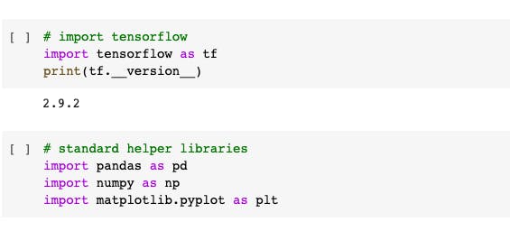
- Import Tensorflow
- Import standard libraries like,
- pandas
- numpy
- matplotlib.pyplot
Getting our data ready
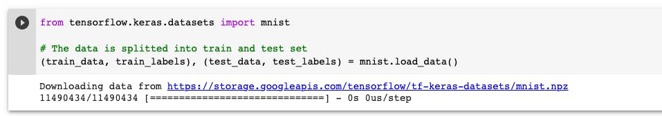
The same MNIST dataset is also available in TensorFlow datasets. Thankfully it's splitted into training and test set which enable us to deep dive directly into exploring and visualizing the data.
Import the data
Let's import the data using tensorflow.keras.datasets library.
Explore the data
Before going further and jumping directly to any step, exploring the data will help us to decide what are the things we need to do with our data, we have to get familiar with data, we have to,
- Find outliers
- If we need a preprocessing phase to uniform
- Check the number of images and labels
- Visualise some numbers
Let's check out the shape of the training and test samples, and observe what it tells.
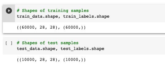
So we have,
- 60000 samples in training data
- 10000 samples in test data
- input is 28 x 28 grayscale image (basically width and height).
Also if we view the data using below code, you might find that the images are in the form of numbers. (you can also try along or refer to Github repo)
train_data[0]
It's in the form of numbers so hardly we can obtain anything by just viewing the numbers in this form, yes we can see that some indexes have 0 as value and in some it's a whole number.
One thing we can do is to plot these and see what they speak.
Visualize the data
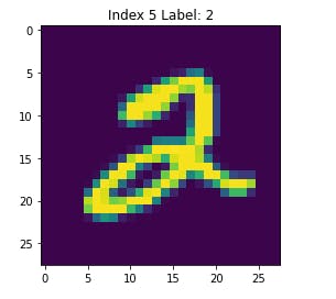
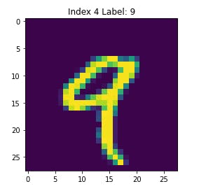
We can plot it using matplotlib since the values that shown above are in the form of array of numbers which has shape (1, 28, 28) of single data.
Use
plt.imshow(train_data[index])
for plotting the images. Here index would be any starting from 0 to upto the length of training samples we have.
So it'll display something like this, if I don't set any color map.
Let's identify how many labels we have in our training set and their corresponding images.

It says, Digit 1 has 6742 samples, 2 has 5958, 3 has 6131 samples and so on... available in training dataset.
These are basically our classnames for multi-class classification problem. Hence, we should store all the classnames into one variable as class_names for further use.
I think we are good with our data and got ourselves familiar with it. So shall we start building our beautiful neural network model ?
Oh Wait, I think we missed one key practice of splitting our data into 3 sets.
Split the data into 3 set (Training, Validation and Test)
It's a good practice in order to build our model, we should split the samples into 3 sets, (Training, Validation and Test set).
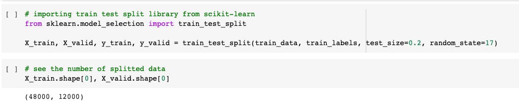
Since we already have the test set available, so we only need to divide the validation test which we split it from training samples.
- Training Samples : (48K)
- Validation Samples : (12K)
- Test Samples : (10K)
We can split the training samples into train and validation samples in many ways but let's use scikit-learn library train_test_split for this.
Awesome, now we're ready to build our neural network model.
Modelling
We're dealing with Multi-class classification problem, so we might need to take care of few things to build our neural network model, but let's start with a basic one to understand the flow.
Default Model
We can start with a very default modelling with default parameters.
Before creating a model, we should set the random seed, so that we can reproduce the same results as many times we want.
tf.random.set_seed(17) // you can choose any number I chose 17.
1. Creating a model: piece together the layers of neural network(using the functional or Sequential API) or import a previously built model(known as transfer learning).
- Input shape: We will have to deal with 28 x 28 tensors (height and width of an image)
- Output shape: 10, since we have 10
class_names(digits) to identify - Input Activation function: Since this is non-linear data, se we'll use non-linear activations like reLu, Softmax, Sigmoid
- Output Activation function: For classification problems, two common functions are Sigmoid and Softmax, since this is a multi-class so we should use Softmax
- Softmax : It converts all the output vector into probabilities that the sum of all the probabilities is equal to 1. Kind of argmax, but softer version.
model_1 = tf.keras.Sequential([
    tf.keras.layers.Flatten(input_shape=(28, 28)), // input shape define
    tf.keras.layers.Dense(4, activation='relu'), // Hidden layer 1 with 4 neurons
    tf.keras.layers.Dense(4, activation='relu'), // Hidden layer 2 with 4 neurons
    tf.keras.layers.Dense(10, activation='softmax') // Output layer, since shape is 10 so 10 neurons.
])
2. Compiling a model: defining how a model's performance should be measured(loss/metrics) as well as defining how it should improve(optimizer).
- Loss function: We have to use CategoricalCrossentropy or SparseCategoricalCrossentropy for multi-class classification problem.
- We will use the later, i.e SparseCategoricalCrossentropy since the other one takes encoded inputs, and we are not
one_hotencoding our training data.
- We will use the later, i.e SparseCategoricalCrossentropy since the other one takes encoded inputs, and we are not
- Optimizer: We can choose from SGD or Adam optimizer functions
- Metrics: For a classification problem, there are many metrics but by default let's see accuracy. How accurate our model is performing.
model_1.compile(loss=tf.keras.losses.SparseCategoricalCrossentropy(),
                optimizer=tf.keras.optimizers.Adam(),
                metrics=['accuracy'])
3. Fitting a model: Letting the model try to find patterns in the data
- Epochs : Number of time our model gets a chance to look our training set and learn pattern from it. We're setting here
20.history_1 = model_1.fit(X_train, y_train, epochs = 20, validation_data=(X_valid, y_valid))
After running and around the last epochs, we get some results like this,
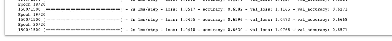
Accuracy on training samples is 66% and loss is fairly low. But we still need to improve our model to get better accuracy.
One more thing we might notice here, val_accuracy, these appears in the process of fitting our model, because we passed a parameter i.e validation_data.
It gives us the idea of how the model performs on validation set during training the model, it gives us the val_loss and val_accuracy.
Anyways, now we got the basic idea, how our model performed with basic settings. We can lift our performance from here by tuning our default model.
Tuning our Model
A model can tuned/improved in many ways but some common ways we can pass through will be,
- Visualize our inputs, if normalization needed then normalize it
- Adjust the layers and activation function
- Tweak optimizer and it's learning rate
- and Many more..
Normalize our inputs
Why do we need to normalize our inputs ?
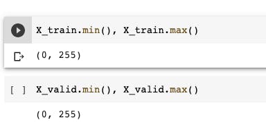
So if we plot the distribution of our images of every pixels, it ranges from 0~255 which is ideally not good for machines to learn the patterns from this spread of distribution.
📖 Quick learn: Why normalization is used to improve deep neural networks ? Check this golden resource
So when we apply normalization, we shrink that spread between 0~1. In our case, if we want to do this we can simply divide all the data with our maximum number i.e 255.
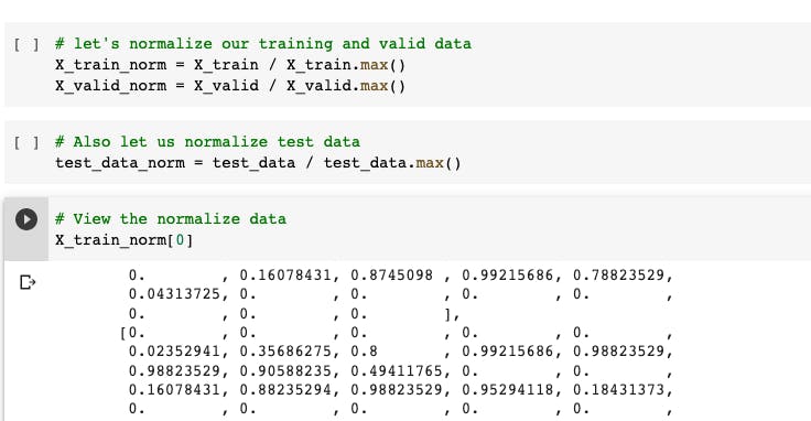
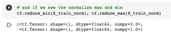
Notice, our images are now normalised and all the numbers ranges from 0~1.
See the numpy value,
Let's build our model again with normalized data. We need to do changes only on fitting step of our model, rest will be the same,
history_2 = model_2.fit(X_train_norm,
                        y_train,
                        epochs = 20,
                        validation_data=(X_valid_norm, y_valid))
Using X_train_norm and X_valid_norm which we have assigned earlier to the normalized inputs.
And if we check the fitting results,

We have increased our Accuracy of model_1 of 66% to 86% of model_2, just by normalizing our data. That's not Bad.
What else we can do to tune our model ?
We can tweak our optimization function.
We have options like SGD(), Adam and many more optimizers, but during experiments I found that Adam performed fairly good but you can try with SGD() as well post the results on comments below.
For now, we can try tweaking some parameters with their different values of one function i.e Adam().
There's a key parameter called, learning_rate, in Adam. It means, how fast the model learn and optimizer function helps it to optimize the learning capabilities.
How about we find the ideal learning rate and see what happens ?
Finding the Ideal learning rate ?
We'll use the same architecture we've been using.
We need to create a callback i.e LearningRateScheduler which takes the current learning rate as the input and returns the next learning rate at the beginning of every epochs.
// Create a learning rate callback
lr_schedular = tf.keras.callbacks.LearningRateScheduler(lambda epoch: 1e-4 * 10**(epoch/20))
Then pass this callback while fitting our model, rest steps will be same,
// Fit the model
history_3 = model_3.fit(X_train_norm,
                        y_train,
                        epochs=80,
                        validation_data=(X_valid_norm, y_valid),
                        callbacks=[lr_schedular])
In this stage, we don't need to bother about the model's accuracy rate or loss. Our goal was to find the ideal learning rate, How we can obtain that ?

Notice we got a new return value lr with some exponential values, those are the different learning rate on which each epoch has run. But let's find out the ideal learning rate.......
By plotting the learning rate decay, and we can write some code for that,
epochs = 80 // we chose 80 epochs to fit our model
lrs = 1e-4 * (10**(tf.range(epochs)/20)) // this is the same lambda variable which we declared with LearningRateScheduler
plt.semilogx(lrs, history_3.history['loss']) // we accessing here the loss value from history that we recieved after fitting the model
plt.xlabel("Learning rate")
plt.ylabel("Loss")
plt.title("Finding the ideal learning rate");
and when plotted, it looks like,
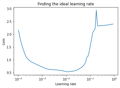
What we learn from the above image ?
It's been observed that, the optimal learning rate is the range between the lowest point in the curve i.e ~0.01 and 10x behind that point i.e ~0.001.
The grey box in the below image shows the ideal learning rate range,
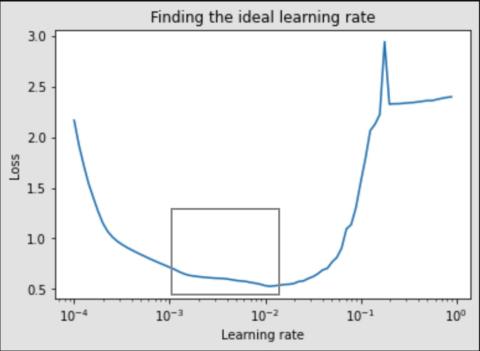
Also 0.001 is the default value of learning_rate of Adam which we have been training our model with these default values so far.
But for completeness lets build our model again with 0.01.
// compile a model
model_4.compile(loss='sparse_categorical_crossentropy',
                optimizer=tf.keras.optimizers.Adam(learning_rate=0.01), // set the learning_rate here
                metrics=['accuracy'])

// fit the model
history_4 = model_4.fit(X_train_norm,
                        y_train,
                        epochs=100, // This time I increased the number of epochs
                        validation_data = (X_valid_norm, y_valid))
And the result of fitting our model_4
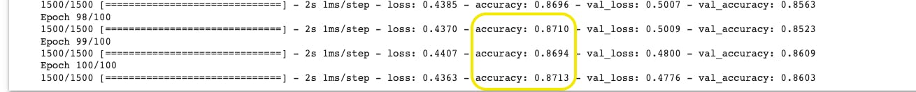
We've trained our model pretty much with an accuracy around of 88% now in Training samples.
But was it because of setting learning rate only ? Not really.
It may be because I let the model to train and learn the patterns for little longer i.e 100 epochs and I think let's increase it a little bit more as 200 epochs and see what happens.
Training the model little longer
Let's increase the number of epochs and the plot the loss (or training) curves to know how did the performance change everytime the model had a change to look at the data (once every epoch) ?
Note: learning_rate is set to default (0.001).
// fit the model
history_5 = model_5.fit(X_train_norm,
                        y_train,
                        epochs=200, // This time for longer period of epochs
                        validation_data = (X_valid_norm, y_valid))
and the results,
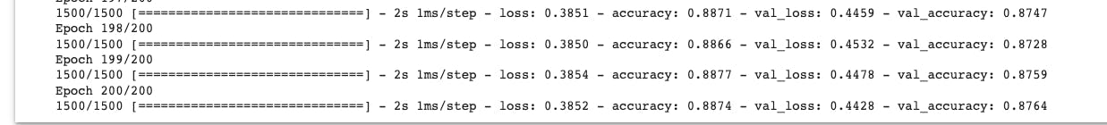
It seems no difference at all. How about plotting the loss curve ?
pd.DataFrame(history_5.history).plot();
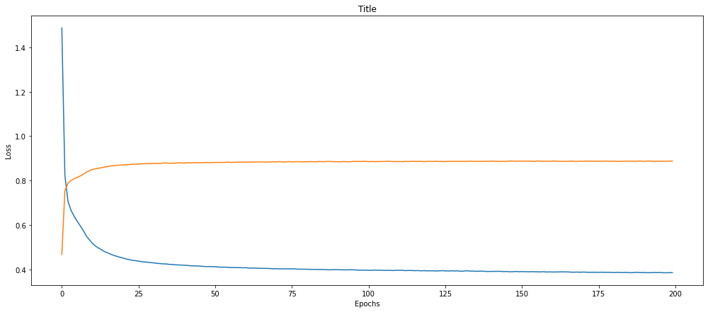
It seems like even we increase the number of epochs the loss will decrease constantly for longer period of time but it'll not drastically decrease upto 0 and and same with the accuracy. May be we can find another way to tune our model and get the higher accuracy.
Let's tweak with Neural Network layers and its units.
Adjusting Neural Network layers and Activation function
- Add more layers, adjust neurons of each layer
- Tweak with different activation functions
Let's see the first one by increasing the number of neurons...
Note : learning_rate is default, epochs is 100.
// create a model
model_6 = tf.keras.Sequential([
    tf.keras.layers.Flatten(input_shape=(28,28)),
    tf.keras.layers.Dense(10, activation='relu'), // before it was 4
    tf.keras.layers.Dense(10, activation='relu'), // before it was 4
    tf.keras.layers.Dense(10, activation='softmax')
])
and now the results are,
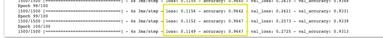
Beautiful ! We almost obtained our goal I guess that our accuracy should reach above 95%.
We can do further experiment and fairly we can tune it little bit more, by adjusting more parameters but since we've set our end goal to achieve 95%. So let's move forward with other things.
Since we have used validation_data while model training so we have the validation accuracy as well which is 93%. Not Bad.
Now, we've covered many things but let's see what more we can do:
- Evaluate it's performance using other classification metrics (or plot confusion matrix)
- Assess some of it's predictions(through visualizations).
- Save and export it for use in an application.
Let's go through first.
Evaluating a model
Important : We'll do all the evaluation on testing set from this stage which means
test_dataandtest_labels.
Confusion matrix
TensorFlow provides a function confusion_matrix() which we can use, but for that we have to make some predictions prior to access that function.
Let's do some predictions,
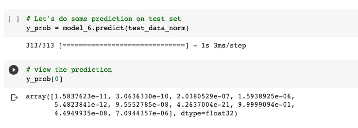
If you notice the data doesn't similar to our test_labels
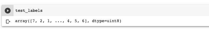
It's because the response that we got from model.predict() are prediction probabilities which we got from our output layer.
So to get our actual prediction similar to the test_labels we need to use argmax().
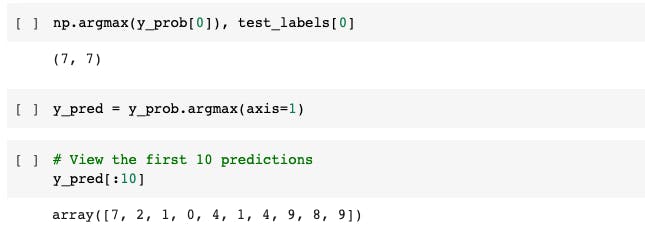 Yeah ! Now we have the same format as in our
 test_labels.
Let's plot the confusion matrix using default confusion matrix provided by TensorFlow.
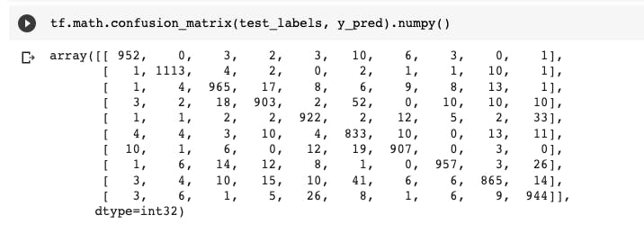
But this doesn't speak much about the thing between predictions and truth labels. For that let's make it little prettier using our custom made function. (Please refer the Github repo for the function)
After plotting the confusion matrix using our custom made function,
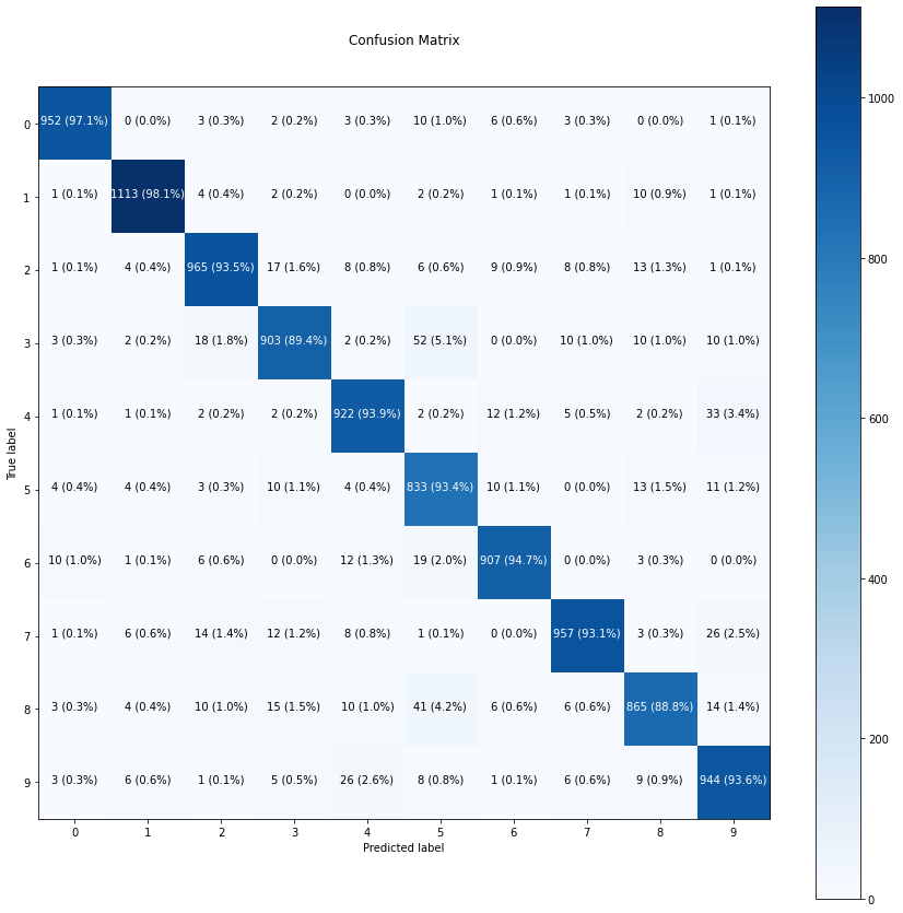
Voila !
It's says, for predicting 0, the accuracy is 97%. for prediction 7, the accuracy is 93% and so on...
Also the color bar tells that, darker the block, the more confident model, in predicting those images or digits.
Next, we do a lot of stuff like evaluating with different metrics and visualising the test results with some random images, saving the model for production use and much more... But let's keep those things for other blogs.
I've try to touch few basic concepts while building a Deep Learning model using a mnist dataset from TensorFlow. Hope you like it. Thanks for reading.
Till then,
Keep Building Yourself 🦾