Introduction

A brit-mathematician, Clive Humby coined a phrase more than a decade ago "\(Data\) \(is\) \(the\) \(New\) \(Oil\)".

Undoubtedly, data is no less than an asset now. Many big companies are dealing with those data and making billions out of them, but do they really use this corpus amount of data in a very raw form, sometimes those data isn't worth a penny if not in a form of something meaningful and valuable.

I'll try to quote a para I read from a blogpost and might also be helpful for you to understand it better,

Data is the new oil. Like oil, data is valuable, but if unrefined it cannot really be used. It has to be changed into gas, plastic, chemicals, etc. to create a valuable entity that drives profitable activity. so, must data be broken down, analysed for it to have value.

And, one of the major ingredient for building a Machine learning model, is data. If that data is not in form of something how machine want it to be, then they might treat the data as gibberish, hard to understand for them, and hence will produce awkward results.

(I think that would be enough to explain the plot of this blog 😅)

Techniques Involved

So there are some techniques to convert those noisy, missing and corrupted data into something meaningful which machine understand, interpret it and produce something meaningful that we, humans could understand and create something out of it.

Data preprocessing includes the steps and techniques we follow to transform those data into something that machine can easily parse it and improve the quality of the data.

Quality results produced from Quality data.

This is one of the phase in the Machine Learning Workflow after gathering our data, we preprocess it and then prepare it for modelling.

Below are some common techniques which is used in most of machine learning projects to preprocess the raw data :

Feature Engineering or Encoding

As we know that, since the beginning of machines era, it communicates with us through binary, whatever we type through our keyboard and give instructions to them the interpreter convert those instructions into \(0s\) and \(1s\), but when huge datasets are prepared using from various data warehouses, those data are in form of string, texts, images, audios, videos or in any other format.

So the processes of converting non-numerical values to numerical values is called as feature encoding.

There are several types of encoding techniques used in Machine Learning process for data preprocessing, some of them are, One Hot Encoding, Label Encoding, Frequency Encoding and Mean Encoding.

Suppose I've a dataset of car sales, and through that dataset I've to build a model which can predict car sale price,

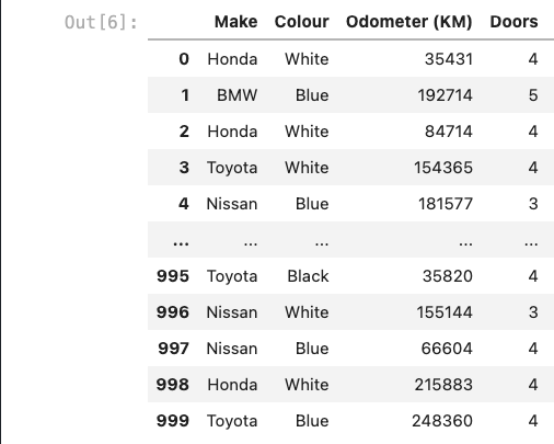
Given, Odometer is numeric type, Make and Colour is non-numeric data type, Doors is a numeric type but a categorical data type.

One Hot Encoding

This technique is often used when categorical non-numeric data exist in our dataset, simply say, to transform categorical non-numerical data into numeric 0 or 1, we use One Hot Encoding technique.

In this method, each category is mapped into separate column that contains 0 or 1 denoting the presence of the feature exist or not.

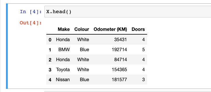
Suppose in the given dataset, we have the values of Colour as White, Blue and Make as Honda, BMW, Toyota, Nissan, then using OneHotEncoder class from scikit-learn,

Before

OneHotEncoder Applied

// Turn the categories into numbers

from sklearn.preprocessing import OneHotEncoder
from sklearn.compose import ColumnTransformer

one_hot = OneHotEncoder()
categorical_feature = ['Make','Colour','Doors']

// Here Doors are also a categorical feature, since some cars have 4 doors, some have 5 and some have 3

transformer = ColumnTransformer([('one_hot', one_hot, categorical_feature)], remainder='passthrough')

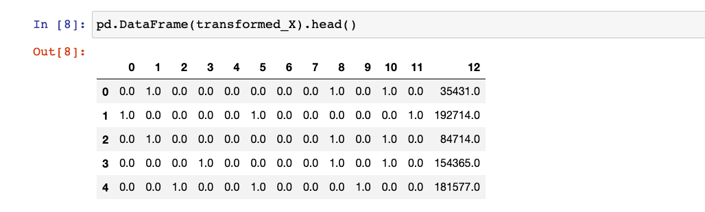
transformed_X = transformer.fit_transform(X)

After

I've covered One Hot Encoding technique only, all other techniques require a separate blog as it would be overwhelming to read in one go.

Let's continue with other steps of data preprocessing👇🏽

Data Imputation

The practice of filling the missing "data" is called as Data Imputation. In statistics, the word imputation means the process of replacing missing data with substituted values.

There are several techniques used in machine learning problem to fill the missing values, but mainly when used Python libraries for machine learning, most commonly used are,

Statistical Imputation (using pandas)

Statistical imputation is an approach of filling the missing data using methods available in statistics such as \(mean()\), \(mode()\), \(median()\) etc.

These are very simple to use and also proven to be very effective in many cases depend on the dataset.

Taking the example of above car sales datasets, for string data types we can impute them with "missing" constant values, for numeric datatype like in our case we can impute with mean() and for categorical like Doors we can use a constant as 4 as all the cars have at least 4 doors.

Using pandas library, the imputation can be done as,

// Fill the data for "Make" column
car_sales["Make"].fillna("missing", inplace=True)

// Fill the data for "Colour" column
car_sales["Colour"].fillna("missing", inplace=True)

// Fill the data for "Odometer (KM)" column
car_sales["Odometer (KM)"].fillna(car_sales_missing["Odometer (KM)"].mean(), inplace=True)

// Fill the data for "Doors" column, since most of the cars have 4 doors so filling with 4
car_sales["Doors"].fillna(4, inplace=True)

Imputation with SimpleImputer (using scikit-learn)

The scikit-learn machine learning library provides the SimpleImputer class, and it provides basic strategies for imputing missing values.

Taking the same dataset of car sales, we can impute the missing values like,

 // We can do the imputation data now using sklearn,

from sklearn.impute import SimpleImputer
from sklearn.compose import ColumnTransformer

// 1. Define columns

cat_features = ['Make', 'Colour']
cat_num_features = ['Doors']
num_features = ["Odometer (KM)"]

// 2. Imputing the missing data

cat_imputer = SimpleImputer(strategy="constant",fill_value="missing")
cat_num_imputer = SimpleImputer(strategy="constant", fill_value=4)
num_imputer = SimpleImputer(strategy="mean")

// 3. Create an imputer that fills missing data

imputer = ColumnTransformer([("cat_imputer", cat_imputer, cat_features),
                             ("cat_num_imputer", cat_num_imputer, cat_num_features),
                             ("num_imputer", num_imputer, num_features)])

This is important to remember that, there's no perfect way to fill the missing data. The methods discussed above are only one of many. The techniques we use will depend on our dataset. I strongly recommend to look for data imputation techniques for further exploration on this topic.

Feature Scaling

Feature scaling is the technique used to make all the numerical values in the same scale.

For example, in our dataset, We are trying to predict the price of a car on the basis of Odometer (KM) which ranges from 6000 KM to 345000 KM, and the median() of previous repair cost varies from 100 to 1700 USD. A machine learning algorithm may have trouble in finding the patterns in these wide-ranging variables.

To fix this, we have two main types of feature scaling,

Normalisation (min-max normalisation)

Normalisation is a technique which makes the feature variables or the values in the columns more consistent with each other, and allows the model to predict outputs more accurately.

It makes the model training less sensitive to the scale of features.

This technique re-scales a feature or observation value with distribution value between 0 and 1.

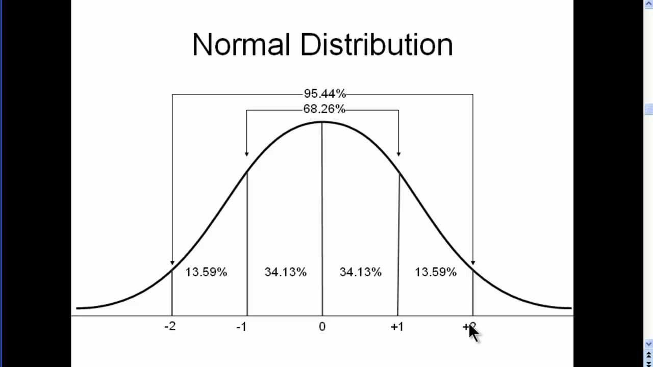
Suppose if we check the distribution of our car-sales Odometer (KM) by plotting it will look like this,

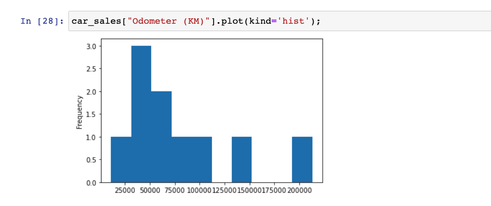
But, when the features are in same scale then after normalisation the normal distribution plot should look like,

Scikit-learn library provides a class called preprocessing which have the utility MinMaxScaler which can be used for scaling into a given range.

Standardisation (z-score normalisation)

This technique is also used to re-scale feature value with the distribution value between 0 and 1, and useful for the optimisation of algorithms, such as gradient descent, for regression and neural network models.

But the main difference is that, we obtain smaller standard deviations through the process of Normalisation as compared to Standardisation.

Scikit-learn library provides a separate utility class to achieve this, preprocessing.StandardScalar

Note

1. Feature scaling usually isn't required for the target variable
2. Feature scaling is usually not required with tree-based models (eg. RandomForest) since they can handle varying features.
3. Feature scaling is very vast topic and differ on the type of machine learning model used, so I'll write a separate blog to cover When to use Normalisation and when Standardisation in coming blogs.

Final Thoughts

I've tried to explain here using some example of structured data, which is in form of tables and spreadsheets. These techniques can also be used for unstructured data like images, audios, documents as well but there are some better techniques available for those data types like converting them into Tensors using Tensorflow which I'll cover those in Deep Learning blogs.

Important Note !

All the techniques that are discussed above must be followed separately for each set of data, which means first the data must be divided into 3 set (training, validation and test) and then these techniques should be applied for each set, or else we might see discrepancies in the patterns that machine learn.

Thanks for reading !

Keep Building 🦾

Cover Photo by Claudio Schwarz on Unsplash